Introduction to the example dataset and file type
Overview
Teaching: 15 min
Exercises: 0 minQuestions
What data are we using in the lesson?
What are VCF files?
Objectives
Know what the example dataset represents
Know the concepts of how VCF files are generated
Preface
The Intro to R and RStudio for Genomics is a part of the Genomics Data Carpentry lessons. In this lesson we will learn the necessary skill sets for R and RStudio and apply them directly to a real next-generation sequencing (NGS) data in the variant calling format (VCF) file type. Previous Genomics Data Carpentry lessons teach learners how to generate a VCF file from FASTQ files downloaded from NCBI Sequence Read Archive (SRA), so we won’t cover that here. Instead, in this episode we will give a brief overview of the data and a what VCF file types are for those who wish to teach the Intro to R and RStudio for Genomics lesson independently of the Genomics Data Carpentry lessons.
This dataset was selected for several reasons, including:
- Simple, but iconic NGS-problem: Examine a population where we want to characterize changes in sequence a priori
- Dataset publicly available - in this case through the NCBI SRA (http://www.ncbi.nlm.nih.gov/sra)
Introduction to the dataset
Microbes are ideal organisms for exploring ‘Long-term Evolution Experiments’ (LTEEs) - thousands of generations can be generated and stored in a way that would be virtually impossible for more complex eukaryotic systems. In Tenaillon et al 2016, 12 populations of Escherichia coli were propagated for more than 50,000 generations in a glucose-limited minimal medium. This medium was supplemented with citrate which E. coli cannot metabolize in the aerobic conditions of the experiment. Sequencing of the populations at regular time points reveals that spontaneous citrate-using mutants (Cit+) appeared in a population of E.coli (designated Ara-3) at around 31,000 generations. It should be noted that spontaneous Cit+ mutants are extraordinarily rare - inability to metabolize citrate is one of the defining characters of the E. coli species. Eventually, Cit+ mutants became the dominant population as the experimental growth medium contained a high concentration of citrate relative to glucose. Around the same time that this mutation emerged, another phenotype become prominent in the Ara-3 population. Many E. coli began to develop excessive numbers of mutations, meaning they became hypermutable.
Strains from generation 0 to generation 50,000 were sequenced, including ones that were both Cit+ and Cit- and hypermutable in later generations.
For the purposes of this workshop we’re going to be working with 3 of the sequence reads from this experiment.
| SRA Run Number | Clone | Generation | Cit | Hypermutable | Read Length | Sequencing Depth |
|---|---|---|---|---|---|---|
| SRR2589044 | REL2181A | 5,000 | Unknown | None | 150 | 60.2 |
| SRR2584863 | REL7179B | 15,000 | Unknown | None | 150 | 88 |
| SRR2584866 | REL11365 | 50,000 | Cit+ | plus | 150 | 138.3 |
We want to be able to look at differences in mutation rates between hypermutable and non-hypermutable strains. We also want to analyze the sequences to figure out what changes occurred in genomes to make the strains Cit+. Ultimately, we will use R to answer the questions:
- How many base pair changes are there between the Cit+ and Cit- strains?
- What are the base pair changes between strains?
How VCF files are generated
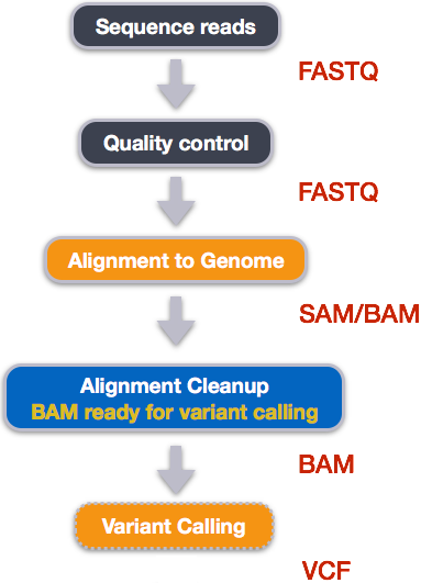
Publicly accessible sequencing files in FASTQ formats can be downloaded from NCBI SRA. However, at FASTQ files contain unaligned sequences of varying quality, and requires clean up and alignment steps for variants to be called from the reference genome.
Five steps are taken to transform FASTQ files to variant calls contained in VCF files and at each step, specialized non-R based bioinformatics tools that are used:
How variant calls are stored in VCF files
VCF files contain variants that were called against a reference genome. These files are slightly more complicated than regular tables you can open using programs like Excel and contain two sections: header and records.
Below you will see the header (which describes the format), the time and date the file was created, the version of bcftools that was used, the command line parameters used, and some additional information:
##fileformat=VCFv4.2
##FILTER=<ID=PASS,Description="All filters passed">
##bcftoolsVersion=1.8+htslib-1.8
##bcftoolsCommand=mpileup -O b -o results/bcf/SRR2584866_raw.bcf -f data/ref_genome/ecoli_rel606.fasta results/bam/SRR2584866.aligned.sorted.bam
##reference=file://data/ref_genome/ecoli_rel606.fasta
##contig=<ID=CP000819.1,length=4629812>
##ALT=<ID=*,Description="Represents allele(s) other than observed.">
##INFO=<ID=INDEL,Number=0,Type=Flag,Description="Indicates that the variant is an INDEL.">
##INFO=<ID=IDV,Number=1,Type=Integer,Description="Maximum number of reads supporting an indel">
##INFO=<ID=IMF,Number=1,Type=Float,Description="Maximum fraction of reads supporting an indel">
##INFO=<ID=DP,Number=1,Type=Integer,Description="Raw read depth">
##INFO=<ID=VDB,Number=1,Type=Float,Description="Variant Distance Bias for filtering splice-site artefacts in RNA-seq data (bigger is better)",Version=
##INFO=<ID=RPB,Number=1,Type=Float,Description="Mann-Whitney U test of Read Position Bias (bigger is better)">
##INFO=<ID=MQB,Number=1,Type=Float,Description="Mann-Whitney U test of Mapping Quality Bias (bigger is better)">
##INFO=<ID=BQB,Number=1,Type=Float,Description="Mann-Whitney U test of Base Quality Bias (bigger is better)">
##INFO=<ID=MQSB,Number=1,Type=Float,Description="Mann-Whitney U test of Mapping Quality vs Strand Bias (bigger is better)">
##INFO=<ID=SGB,Number=1,Type=Float,Description="Segregation based metric.">
##INFO=<ID=MQ0F,Number=1,Type=Float,Description="Fraction of MQ0 reads (smaller is better)">
##FORMAT=<ID=PL,Number=G,Type=Integer,Description="List of Phred-scaled genotype likelihoods">
##FORMAT=<ID=GT,Number=1,Type=String,Description="Genotype">
##INFO=<ID=ICB,Number=1,Type=Float,Description="Inbreeding Coefficient Binomial test (bigger is better)">
##INFO=<ID=HOB,Number=1,Type=Float,Description="Bias in the number of HOMs number (smaller is better)">
##INFO=<ID=AC,Number=A,Type=Integer,Description="Allele count in genotypes for each ALT allele, in the same order as listed">
##INFO=<ID=AN,Number=1,Type=Integer,Description="Total number of alleles in called genotypes">
##INFO=<ID=DP4,Number=4,Type=Integer,Description="Number of high-quality ref-forward , ref-reverse, alt-forward and alt-reverse bases">
##INFO=<ID=MQ,Number=1,Type=Integer,Description="Average mapping quality">
##bcftools_callVersion=1.8+htslib-1.8
##bcftools_callCommand=call --ploidy 1 -m -v -o results/bcf/SRR2584866_variants.vcf results/bcf/SRR2584866_raw.bcf; Date=Tue Oct  9 18:48:10 2018
Followed by information on each of the variations observed:
#CHROM  POS     ID      REF     ALT     QUAL    FILTER  INFO    FORMAT  results/bam/SRR2584866.aligned.sorted.bam
CP000819.1      1521    .       C       T       207     .       DP=9;VDB=0.993024;SGB=-0.662043;MQSB=0.974597;MQ0F=0;AC=1;AN=1;DP4=0,0,4,5;MQ=60
CP000819.1      1612    .       A       G       225     .       DP=13;VDB=0.52194;SGB=-0.676189;MQSB=0.950952;MQ0F=0;AC=1;AN=1;DP4=0,0,6,5;MQ=60
CP000819.1      9092    .       A       G       225     .       DP=14;VDB=0.717543;SGB=-0.670168;MQSB=0.916482;MQ0F=0;AC=1;AN=1;DP4=0,0,7,3;MQ=60
CP000819.1      9972    .       T       G       214     .       DP=10;VDB=0.022095;SGB=-0.670168;MQSB=1;MQ0F=0;AC=1;AN=1;DP4=0,0,2,8;MQ=60      GT:PL
CP000819.1      10563   .       G       A       225     .       DP=11;VDB=0.958658;SGB=-0.670168;MQSB=0.952347;MQ0F=0;AC=1;AN=1;DP4=0,0,5,5;MQ=60
CP000819.1      22257   .       C       T       127     .       DP=5;VDB=0.0765947;SGB=-0.590765;MQSB=1;MQ0F=0;AC=1;AN=1;DP4=0,0,2,3;MQ=60      GT:PL
CP000819.1      38971   .       A       G       225     .       DP=14;VDB=0.872139;SGB=-0.680642;MQSB=1;MQ0F=0;AC=1;AN=1;DP4=0,0,4,8;MQ=60      GT:PL
CP000819.1      42306   .       A       G       225     .       DP=15;VDB=0.969686;SGB=-0.686358;MQSB=1;MQ0F=0;AC=1;AN=1;DP4=0,0,5,9;MQ=60      GT:PL
CP000819.1      45277   .       A       G       225     .       DP=15;VDB=0.470998;SGB=-0.680642;MQSB=0.95494;MQ0F=0;AC=1;AN=1;DP4=0,0,7,5;MQ=60
CP000819.1      56613   .       C       G       183     .       DP=12;VDB=0.879703;SGB=-0.676189;MQSB=1;MQ0F=0;AC=1;AN=1;DP4=0,0,8,3;MQ=60      GT:PL
CP000819.1      62118   .       A       G       225     .       DP=19;VDB=0.414981;SGB=-0.691153;MQSB=0.906029;MQ0F=0;AC=1;AN=1;DP4=0,0,8,10;MQ=59
CP000819.1      64042   .       G       A       225     .       DP=18;VDB=0.451328;SGB=-0.689466;MQSB=1;MQ0F=0;AC=1;AN=1;DP4=0,0,7,9;MQ=60      GT:PL
The first few columns represent the information we have about a predicted variation.
| column | info |
|---|---|
| CHROM | contig location where the variation occurs |
| POS | position within the contig where the variation occurs |
| ID | a . until we add annotation information |
| REF | reference genotype (forward strand) |
| ALT | sample genotype (forward strand) |
| QUAL | Phred-scaled probability that the observed variant exists at this site (higher is better) |
| FILTER | a . if no quality filters have been applied, PASS if a filter is passed, or the name of the filters this variant failed |
In an ideal world, the information in the QUAL column would be all we needed to filter out bad variant calls.
However, in reality we need to filter on multiple other metrics.
The last two columns contain the genotypes and can be tricky to decode.
| column | info |
|---|---|
| FORMAT | lists in order the metrics presented in the final column |
| results | lists the values associated with those metrics in order |
For our file, the metrics presented are GT:PL:GQ.
| metric | definition |
|---|---|
| AD, DP | the depth per allele by sample and coverage |
| GT | the genotype for the sample at this loci. For a diploid organism, the GT field indicates the two alleles carried by the sample, encoded by a 0 for the REF allele, 1 for the first ALT allele, 2 for the second ALT allele, etc. A 0/0 means homozygous reference, 0/1 is heterozygous, and 1/1 is homozygous for the alternate allele. |
| PL | the likelihoods of the given genotypes |
| GQ | the Phred-scaled confidence for the genotype |
For more information on VCF files visit The Broad Institute’s VCF guide.
References
Tenaillon O, Barrick JE, Ribeck N, Deatherage DE, Blanchard JL, Dasgupta A, Wu GC, Wielgoss S, Cruveiller S, Médigue C, Schneider D, Lenski RE. Tempo and mode of genome evolution in a 50,000-generation experiment (2016) Nature. 536(7615): 165–170. Paper, Supplemental materials Data on NCBI SRA: https://trace.ncbi.nlm.nih.gov/Traces/sra/?study=SRP064605 Data on EMBL-EBI ENA: https://www.ebi.ac.uk/ena/data/view/PRJNA295606
This episode was adapted from the Data Carpentry Genomic lessons:
Key Points
The dataset comes from a real world experiment in E. coli.
Publicly available FASTQ files can be downloaded from NCBI SRA.
Several steps are taken outside of R/RStudio to create VCF files from FASTQ files.
VCF files store variant calls in a special format.