Data Wrangling and Analyses with Tidyverse

Overview

Teaching: 40 min
Exercises: 15 min

Questions

How can I manipulate data frames without repeating myself?

Objectives

Describe what the dplyr package in R is used for.

Apply common dplyr functions to manipulate data in R.

Employ the ‘pipe’ operator to link together a sequence of functions.

Employ the ‘mutate’ function to apply other chosen functions to existing columns and create new columns of data.

Employ the ‘split-apply-combine’ concept to split the data into groups, apply analysis to each group, and combine the results.

Bracket subsetting is handy, but it can be cumbersome and difficult to read, especially for complicated operations.

Luckily, the dplyr package provides a number of very useful functions for manipulating data frames in a way that will reduce repetition, reduce the probability of making errors, and probably even save you some typing. As an added bonus, you might even find the dplyr grammar easier to read.

Here we’re going to cover some of the most commonly used functions as well as using pipes (%>%) to combine them:

glimpse()
select()
filter()
group_by()
summarize()
mutate()
pivot_longer and pivot_wider

Packages in R are sets of additional functions that let you do more stuff in R. The functions we’ve been using, like str(), come built into R; packages give you access to more functions. You need to install a package and then load it to be able to use it.

install.packages("dplyr") ## install

You might get asked to choose a CRAN mirror – this is asking you to choose a site to download the package from. The choice doesn’t matter too much; I’d recommend choosing the RStudio mirror.

library("dplyr")          ## load

You only need to install a package once per computer, but you need to load it every time you open a new R session and want to use that package.

What is dplyr?

The package dplyr is a fairly new (2014) package that tries to provide easy tools for the most common data manipulation tasks. This package is also included in the tidyverse package, which is a collection of eight different packages (dplyr, ggplot2, tibble, tidyr, readr, purrr, stringr, and forcats). It is built to work directly with data frames. The thinking behind it was largely inspired by the package plyr which has been in use for some time but suffered from being slow in some cases. dplyr addresses this by porting much of the computation to C++. An additional feature is the ability to work with data stored directly in an external database. The benefits of doing this are that the data can be managed natively in a relational database, queries can be conducted on that database, and only the results of the query returned.

This addresses a common problem with R in that all operations are conducted in memory and thus the amount of data you can work with is limited by available memory. The database connections essentially remove that limitation in that you can have a database that is over 100s of GB, conduct queries on it directly and pull back just what you need for analysis in R.

Taking a quick look at data frames

Similar to str(), which comes built into R, glimpse() is a dplyr function that (as the name suggests) gives a glimpse of the data frame.

Rows: 801
Columns: 29
$ sample_id     <chr> "SRR2584863", "SRR2584863", "SRR2584863", "SRR2584863", …
$ CHROM         <chr> "CP000819.1", "CP000819.1", "CP000819.1", "CP000819.1", …
$ POS           <dbl> 9972, 263235, 281923, 433359, 473901, 648692, 1331794, 1…
$ ID            <lgl> NA, NA, NA, NA, NA, NA, NA, NA, NA, NA, NA, NA, NA, NA, …
$ REF           <chr> "T", "G", "G", "CTTTTTTT", "CCGC", "C", "C", "G", "ACAGC…
$ ALT           <chr> "G", "T", "T", "CTTTTTTTT", "CCGCGC", "T", "A", "A", "AC…
$ QUAL          <dbl> 91.0000, 85.0000, 217.0000, 64.0000, 228.0000, 210.0000,…
$ FILTER        <lgl> NA, NA, NA, NA, NA, NA, NA, NA, NA, NA, NA, NA, NA, NA, …
$ INDEL         <lgl> FALSE, FALSE, FALSE, TRUE, TRUE, FALSE, FALSE, FALSE, TR…
$ IDV           <dbl> NA, NA, NA, 12, 9, NA, NA, NA, 2, 7, NA, NA, NA, NA, NA,…
$ IMF           <dbl> NA, NA, NA, 1.000000, 0.900000, NA, NA, NA, 0.666667, 1.…
$ DP            <dbl> 4, 6, 10, 12, 10, 10, 8, 11, 3, 7, 9, 20, 12, 19, 15, 10…
$ VDB           <dbl> 0.0257451, 0.0961330, 0.7740830, 0.4777040, 0.6595050, 0…
$ RPB           <dbl> NA, 1.000000, NA, NA, NA, NA, NA, NA, NA, NA, 0.900802, …
$ MQB           <dbl> NA, 1.0000000, NA, NA, NA, NA, NA, NA, NA, NA, 0.1501340…
$ BQB           <dbl> NA, 1.000000, NA, NA, NA, NA, NA, NA, NA, NA, 0.750668, …
$ MQSB          <dbl> NA, NA, 0.974597, 1.000000, 0.916482, 0.916482, 0.900802…
$ SGB           <dbl> -0.556411, -0.590765, -0.662043, -0.676189, -0.662043, -…
$ MQ0F          <dbl> 0.000000, 0.166667, 0.000000, 0.000000, 0.000000, 0.0000…
$ ICB           <lgl> NA, NA, NA, NA, NA, NA, NA, NA, NA, NA, NA, NA, NA, NA, …
$ HOB           <lgl> NA, NA, NA, NA, NA, NA, NA, NA, NA, NA, NA, NA, NA, NA, …
$ AC            <dbl> 1, 1, 1, 1, 1, 1, 1, 1, 1, 1, 1, 1, 1, 1, 1, 1, 1, 1, 1,…
$ AN            <dbl> 1, 1, 1, 1, 1, 1, 1, 1, 1, 1, 1, 1, 1, 1, 1, 1, 1, 1, 1,…
$ DP4           <chr> "0,0,0,4", "0,1,0,5", "0,0,4,5", "0,1,3,8", "1,0,2,7", "…
$ MQ            <dbl> 60, 33, 60, 60, 60, 60, 60, 60, 60, 60, 25, 60, 10, 60, …
$ Indiv         <chr> "/home/dcuser/dc_workshop/results/bam/SRR2584863.aligned…
$ gt_PL         <dbl> 1210, 1120, 2470, 910, 2550, 2400, 2080, 2550, 11128, 19…
$ gt_GT         <dbl> 1, 1, 1, 1, 1, 1, 1, 1, 1, 1, 1, 1, 1, 1, 1, 1, 1, 1, 1,…
$ gt_GT_alleles <chr> "G", "T", "T", "CTTTTTTTT", "CCGCGC", "T", "A", "A", "AC…

In the above output, we can already gather some information about variants, such as the number of rows and columns, column names, type of vector in the columns, and the first few entries of each column. Although what we see is similar to outputs of str(), this method gives a cleaner visual output.

Selecting columns and filtering rows

To select columns of a data frame, use select(). The first argument to this function is the data frame (variants), and the subsequent arguments are the columns to keep.

select(variants, sample_id, REF, ALT, DP)

# A tibble: 801 × 4
   sample_id  REF                              ALT                            DP
   <chr>      <chr>                            <chr>                       <dbl>
SRR2584863 T                                G                               4
SRR2584863 G                                T                               6
SRR2584863 G                                T                              10
SRR2584863 CTTTTTTT                         CTTTTTTTT                      12
SRR2584863 CCGC                             CCGCGC                         10
SRR2584863 C                                T                              10
SRR2584863 C                                A                               8
SRR2584863 G                                A                              11
SRR2584863 ACAGCCAGCCAGCCAGCCAGCCAGCCAGCCAG ACAGCCAGCCAGCCAGCCAGCCAGCC…     3
SRR2584863 AT                               ATT                             7
# … with 791 more rows

To select all columns except certain ones, put a “-“ in front of the variable to exclude it.

select(variants, -CHROM)

# A tibble: 801 × 28
   sample_id      POS ID    REF      ALT    QUAL FILTER INDEL   IDV    IMF    DP
   <chr>        <dbl> <lgl> <chr>    <chr> <dbl> <lgl>  <lgl> <dbl>  <dbl> <dbl>
 1 SRR2584863    9972 NA    T        G        91 NA     FALSE    NA NA         4
 2 SRR2584863  263235 NA    G        T        85 NA     FALSE    NA NA         6
 3 SRR2584863  281923 NA    G        T       217 NA     FALSE    NA NA        10
 4 SRR2584863  433359 NA    CTTTTTTT CTTT…    64 NA     TRUE     12  1        12
 5 SRR2584863  473901 NA    CCGC     CCGC…   228 NA     TRUE      9  0.9      10
 6 SRR2584863  648692 NA    C        T       210 NA     FALSE    NA NA        10
 7 SRR2584863 1331794 NA    C        A       178 NA     FALSE    NA NA         8
 8 SRR2584863 1733343 NA    G        A       225 NA     FALSE    NA NA        11
 9 SRR2584863 2103887 NA    ACAGCCA… ACAG…    56 NA     TRUE      2  0.667     3
10 SRR2584863 2333538 NA    AT       ATT     167 NA     TRUE      7  1         7
# … with 791 more rows, and 17 more variables: VDB <dbl>, RPB <dbl>, MQB <dbl>,
#   BQB <dbl>, MQSB <dbl>, SGB <dbl>, MQ0F <dbl>, ICB <lgl>, HOB <lgl>,
#   AC <dbl>, AN <dbl>, DP4 <chr>, MQ <dbl>, Indiv <chr>, gt_PL <dbl>,
#   gt_GT <dbl>, gt_GT_alleles <chr>

dplyr also provides useful functions to select columns based on their names. For instance, ends_with() allows you to select columns that ends with specific letters. For instance, if you wanted to select columns that end with the letter “B”:

select(variants, ends_with("B"))

# A tibble: 801 × 8
      VDB   RPB   MQB   BQB   MQSB    SGB ICB   HOB  
    <dbl> <dbl> <dbl> <dbl>  <dbl>  <dbl> <lgl> <lgl>
0.0257    NA    NA    NA NA     -0.556 NA    NA   
0.0961     1     1     1 NA     -0.591 NA    NA   
0.774     NA    NA    NA  0.975 -0.662 NA    NA   
0.478     NA    NA    NA  1     -0.676 NA    NA   
0.660     NA    NA    NA  0.916 -0.662 NA    NA   
0.268     NA    NA    NA  0.916 -0.670 NA    NA   
0.624     NA    NA    NA  0.901 -0.651 NA    NA   
0.992     NA    NA    NA  1.01  -0.670 NA    NA   
0.902     NA    NA    NA  1     -0.454 NA    NA   
0.568     NA    NA    NA  1.01  -0.617 NA    NA   
# … with 791 more rows

Challenge

Create a table that contains all the columns with the letter “i” and column “POS”, without columns “Indiv” and “FILTER”. Hint: look at the help function ends_with() we’ve just covered.

Solution

select(variants, contains("i"), -Indiv, -FILTER, POS)

# A tibble: 801 × 7
   sample_id  ID    INDEL   IDV    IMF ICB       POS
   <chr>      <lgl> <lgl> <dbl>  <dbl> <lgl>   <dbl>
SRR2584863 NA    FALSE    NA NA     NA       9972
SRR2584863 NA    FALSE    NA NA     NA     263235
SRR2584863 NA    FALSE    NA NA     NA     281923
SRR2584863 NA    TRUE     12  1     NA     433359
SRR2584863 NA    TRUE      9  0.9   NA     473901
SRR2584863 NA    FALSE    NA NA     NA     648692
SRR2584863 NA    FALSE    NA NA     NA    1331794
SRR2584863 NA    FALSE    NA NA     NA    1733343
SRR2584863 NA    TRUE      2  0.667 NA    2103887
SRR2584863 NA    TRUE      7  1     NA    2333538
# … with 791 more rows

To choose rows, use filter():

filter(variants, sample_id == "SRR2584863")

# A tibble: 25 × 29
   sample_id  CHROM        POS ID    REF   ALT    QUAL FILTER INDEL   IDV    IMF
   <chr>      <chr>      <dbl> <lgl> <chr> <chr> <dbl> <lgl>  <lgl> <dbl>  <dbl>
 1 SRR2584863 CP000819… 9.97e3 NA    T     G        91 NA     FALSE    NA NA    
 2 SRR2584863 CP000819… 2.63e5 NA    G     T        85 NA     FALSE    NA NA    
 3 SRR2584863 CP000819… 2.82e5 NA    G     T       217 NA     FALSE    NA NA    
 4 SRR2584863 CP000819… 4.33e5 NA    CTTT… CTTT…    64 NA     TRUE     12  1    
 5 SRR2584863 CP000819… 4.74e5 NA    CCGC  CCGC…   228 NA     TRUE      9  0.9  
 6 SRR2584863 CP000819… 6.49e5 NA    C     T       210 NA     FALSE    NA NA    
 7 SRR2584863 CP000819… 1.33e6 NA    C     A       178 NA     FALSE    NA NA    
 8 SRR2584863 CP000819… 1.73e6 NA    G     A       225 NA     FALSE    NA NA    
 9 SRR2584863 CP000819… 2.10e6 NA    ACAG… ACAG…    56 NA     TRUE      2  0.667
10 SRR2584863 CP000819… 2.33e6 NA    AT    ATT     167 NA     TRUE      7  1    
# … with 15 more rows, and 18 more variables: DP <dbl>, VDB <dbl>, RPB <dbl>,
#   MQB <dbl>, BQB <dbl>, MQSB <dbl>, SGB <dbl>, MQ0F <dbl>, ICB <lgl>,
#   HOB <lgl>, AC <dbl>, AN <dbl>, DP4 <chr>, MQ <dbl>, Indiv <chr>,
#   gt_PL <dbl>, gt_GT <dbl>, gt_GT_alleles <chr>

filter() will keep all the rows that match the conditions that are provided. Here are a few examples:

# rows for which the reference genome has T or G
filter(variants, REF %in% c("T", "G"))

# A tibble: 340 × 29
   sample_id CHROM    POS ID    REF   ALT    QUAL FILTER INDEL   IDV   IMF    DP
   <chr>     <chr>  <dbl> <lgl> <chr> <chr> <dbl> <lgl>  <lgl> <dbl> <dbl> <dbl>
 1 SRR25848… CP00… 9.97e3 NA    T     G      91   NA     FALSE    NA    NA     4
 2 SRR25848… CP00… 2.63e5 NA    G     T      85   NA     FALSE    NA    NA     6
 3 SRR25848… CP00… 2.82e5 NA    G     T     217   NA     FALSE    NA    NA    10
 4 SRR25848… CP00… 1.73e6 NA    G     A     225   NA     FALSE    NA    NA    11
 5 SRR25848… CP00… 2.62e6 NA    G     T      31.9 NA     FALSE    NA    NA    12
 6 SRR25848… CP00… 3.00e6 NA    G     A     225   NA     FALSE    NA    NA    15
 7 SRR25848… CP00… 3.91e6 NA    G     T     225   NA     FALSE    NA    NA    10
 8 SRR25848… CP00… 9.97e3 NA    T     G     214   NA     FALSE    NA    NA    10
 9 SRR25848… CP00… 1.06e4 NA    G     A     225   NA     FALSE    NA    NA    11
10 SRR25848… CP00… 6.40e4 NA    G     A     225   NA     FALSE    NA    NA    18
# … with 330 more rows, and 17 more variables: VDB <dbl>, RPB <dbl>, MQB <dbl>,
#   BQB <dbl>, MQSB <dbl>, SGB <dbl>, MQ0F <dbl>, ICB <lgl>, HOB <lgl>,
#   AC <dbl>, AN <dbl>, DP4 <chr>, MQ <dbl>, Indiv <chr>, gt_PL <dbl>,
#   gt_GT <dbl>, gt_GT_alleles <chr>

# rows with QUAL values greater than or equal to 100
filter(variants, QUAL >= 100)

# A tibble: 666 × 29
   sample_id CHROM    POS ID    REF   ALT    QUAL FILTER INDEL   IDV   IMF    DP
   <chr>     <chr>  <dbl> <lgl> <chr> <chr> <dbl> <lgl>  <lgl> <dbl> <dbl> <dbl>
 1 SRR25848… CP00… 2.82e5 NA    G     T       217 NA     FALSE    NA  NA      10
 2 SRR25848… CP00… 4.74e5 NA    CCGC  CCGC…   228 NA     TRUE      9   0.9    10
 3 SRR25848… CP00… 6.49e5 NA    C     T       210 NA     FALSE    NA  NA      10
 4 SRR25848… CP00… 1.33e6 NA    C     A       178 NA     FALSE    NA  NA       8
 5 SRR25848… CP00… 1.73e6 NA    G     A       225 NA     FALSE    NA  NA      11
 6 SRR25848… CP00… 2.33e6 NA    AT    ATT     167 NA     TRUE      7   1       7
 7 SRR25848… CP00… 2.41e6 NA    A     C       104 NA     FALSE    NA  NA       9
 8 SRR25848… CP00… 2.45e6 NA    A     C       225 NA     FALSE    NA  NA      20
 9 SRR25848… CP00… 2.67e6 NA    A     T       225 NA     FALSE    NA  NA      19
10 SRR25848… CP00… 3.00e6 NA    G     A       225 NA     FALSE    NA  NA      15
# … with 656 more rows, and 17 more variables: VDB <dbl>, RPB <dbl>, MQB <dbl>,
#   BQB <dbl>, MQSB <dbl>, SGB <dbl>, MQ0F <dbl>, ICB <lgl>, HOB <lgl>,
#   AC <dbl>, AN <dbl>, DP4 <chr>, MQ <dbl>, Indiv <chr>, gt_PL <dbl>,
#   gt_GT <dbl>, gt_GT_alleles <chr>

# rows that have TRUE in the column INDEL
filter(variants, INDEL)

# A tibble: 101 × 29
   sample_id CHROM    POS ID    REF   ALT    QUAL FILTER INDEL   IDV   IMF    DP
   <chr>     <chr>  <dbl> <lgl> <chr> <chr> <dbl> <lgl>  <lgl> <dbl> <dbl> <dbl>
 1 SRR25848… CP00… 4.33e5 NA    CTTT… CTTT…  64   NA     TRUE     12 1        12
 2 SRR25848… CP00… 4.74e5 NA    CCGC  CCGC… 228   NA     TRUE      9 0.9      10
 3 SRR25848… CP00… 2.10e6 NA    ACAG… ACAG…  56   NA     TRUE      2 0.667     3
 4 SRR25848… CP00… 2.33e6 NA    AT    ATT   167   NA     TRUE      7 1         7
 5 SRR25848… CP00… 3.90e6 NA    A     AC     43.4 NA     TRUE      2 1         2
 6 SRR25848… CP00… 4.43e6 NA    TGG   T     228   NA     TRUE     10 1        10
 7 SRR25848… CP00… 1.48e5 NA    AGGGG AGGG… 122   NA     TRUE      8 1         8
 8 SRR25848… CP00… 1.58e5 NA    GTTT… GTTT…  19.5 NA     TRUE      6 1         6
 9 SRR25848… CP00… 1.73e5 NA    CAA   CA    180   NA     TRUE     11 1        11
10 SRR25848… CP00… 1.75e5 NA    GAA   GA    194   NA     TRUE     10 1        10
# … with 91 more rows, and 17 more variables: VDB <dbl>, RPB <dbl>, MQB <dbl>,
#   BQB <dbl>, MQSB <dbl>, SGB <dbl>, MQ0F <dbl>, ICB <lgl>, HOB <lgl>,
#   AC <dbl>, AN <dbl>, DP4 <chr>, MQ <dbl>, Indiv <chr>, gt_PL <dbl>,
#   gt_GT <dbl>, gt_GT_alleles <chr>

# rows that don't have missing data in the IDV column
filter(variants, !is.na(IDV))

# A tibble: 101 × 29
   sample_id CHROM    POS ID    REF   ALT    QUAL FILTER INDEL   IDV   IMF    DP
   <chr>     <chr>  <dbl> <lgl> <chr> <chr> <dbl> <lgl>  <lgl> <dbl> <dbl> <dbl>
 1 SRR25848… CP00… 4.33e5 NA    CTTT… CTTT…  64   NA     TRUE     12 1        12
 2 SRR25848… CP00… 4.74e5 NA    CCGC  CCGC… 228   NA     TRUE      9 0.9      10
 3 SRR25848… CP00… 2.10e6 NA    ACAG… ACAG…  56   NA     TRUE      2 0.667     3
 4 SRR25848… CP00… 2.33e6 NA    AT    ATT   167   NA     TRUE      7 1         7
 5 SRR25848… CP00… 3.90e6 NA    A     AC     43.4 NA     TRUE      2 1         2
 6 SRR25848… CP00… 4.43e6 NA    TGG   T     228   NA     TRUE     10 1        10
 7 SRR25848… CP00… 1.48e5 NA    AGGGG AGGG… 122   NA     TRUE      8 1         8
 8 SRR25848… CP00… 1.58e5 NA    GTTT… GTTT…  19.5 NA     TRUE      6 1         6
 9 SRR25848… CP00… 1.73e5 NA    CAA   CA    180   NA     TRUE     11 1        11
10 SRR25848… CP00… 1.75e5 NA    GAA   GA    194   NA     TRUE     10 1        10
# … with 91 more rows, and 17 more variables: VDB <dbl>, RPB <dbl>, MQB <dbl>,
#   BQB <dbl>, MQSB <dbl>, SGB <dbl>, MQ0F <dbl>, ICB <lgl>, HOB <lgl>,
#   AC <dbl>, AN <dbl>, DP4 <chr>, MQ <dbl>, Indiv <chr>, gt_PL <dbl>,
#   gt_GT <dbl>, gt_GT_alleles <chr>

filter() allows you to combine multiple conditions. You can separate them using a , as arguments to the function, they will be combined using the & (AND) logical operator. If you need to use the | (OR) logical operator, you can specify it explicitly:

# this is equivalent to:
#   filter(variants, sample_id == "SRR2584863" & QUAL >= 100)
filter(variants, sample_id == "SRR2584863", QUAL >= 100)

# A tibble: 19 × 29
   sample_id CHROM    POS ID    REF   ALT    QUAL FILTER INDEL   IDV   IMF    DP
   <chr>     <chr>  <dbl> <lgl> <chr> <chr> <dbl> <lgl>  <lgl> <dbl> <dbl> <dbl>
SRR25848… CP00… 2.82e5 NA    G     T       217 NA     FALSE    NA  NA      10
SRR25848… CP00… 4.74e5 NA    CCGC  CCGC…   228 NA     TRUE      9   0.9    10
SRR25848… CP00… 6.49e5 NA    C     T       210 NA     FALSE    NA  NA      10
SRR25848… CP00… 1.33e6 NA    C     A       178 NA     FALSE    NA  NA       8
SRR25848… CP00… 1.73e6 NA    G     A       225 NA     FALSE    NA  NA      11
SRR25848… CP00… 2.33e6 NA    AT    ATT     167 NA     TRUE      7   1       7
SRR25848… CP00… 2.41e6 NA    A     C       104 NA     FALSE    NA  NA       9
SRR25848… CP00… 2.45e6 NA    A     C       225 NA     FALSE    NA  NA      20
SRR25848… CP00… 2.67e6 NA    A     T       225 NA     FALSE    NA  NA      19
SRR25848… CP00… 3.00e6 NA    G     A       225 NA     FALSE    NA  NA      15
SRR25848… CP00… 3.34e6 NA    A     C       211 NA     FALSE    NA  NA      10
SRR25848… CP00… 3.40e6 NA    C     A       225 NA     FALSE    NA  NA      14
SRR25848… CP00… 3.48e6 NA    A     G       200 NA     FALSE    NA  NA       9
SRR25848… CP00… 3.49e6 NA    A     C       225 NA     FALSE    NA  NA      13
SRR25848… CP00… 3.91e6 NA    G     T       225 NA     FALSE    NA  NA      10
SRR25848… CP00… 4.10e6 NA    A     G       225 NA     FALSE    NA  NA      16
SRR25848… CP00… 4.20e6 NA    A     C       225 NA     FALSE    NA  NA      11
SRR25848… CP00… 4.43e6 NA    TGG   T       228 NA     TRUE     10   1      10
SRR25848… CP00… 4.62e6 NA    A     C       185 NA     FALSE    NA  NA       9
# … with 17 more variables: VDB <dbl>, RPB <dbl>, MQB <dbl>, BQB <dbl>,
#   MQSB <dbl>, SGB <dbl>, MQ0F <dbl>, ICB <lgl>, HOB <lgl>, AC <dbl>,
#   AN <dbl>, DP4 <chr>, MQ <dbl>, Indiv <chr>, gt_PL <dbl>, gt_GT <dbl>,
#   gt_GT_alleles <chr>

# using `|` logical operator
filter(variants, sample_id == "SRR2584863", (INDEL | QUAL >= 100))

# A tibble: 22 × 29
   sample_id  CHROM        POS ID    REF   ALT    QUAL FILTER INDEL   IDV    IMF
   <chr>      <chr>      <dbl> <lgl> <chr> <chr> <dbl> <lgl>  <lgl> <dbl>  <dbl>
 1 SRR2584863 CP000819… 2.82e5 NA    G     T       217 NA     FALSE    NA NA    
 2 SRR2584863 CP000819… 4.33e5 NA    CTTT… CTTT…    64 NA     TRUE     12  1    
 3 SRR2584863 CP000819… 4.74e5 NA    CCGC  CCGC…   228 NA     TRUE      9  0.9  
 4 SRR2584863 CP000819… 6.49e5 NA    C     T       210 NA     FALSE    NA NA    
 5 SRR2584863 CP000819… 1.33e6 NA    C     A       178 NA     FALSE    NA NA    
 6 SRR2584863 CP000819… 1.73e6 NA    G     A       225 NA     FALSE    NA NA    
 7 SRR2584863 CP000819… 2.10e6 NA    ACAG… ACAG…    56 NA     TRUE      2  0.667
 8 SRR2584863 CP000819… 2.33e6 NA    AT    ATT     167 NA     TRUE      7  1    
 9 SRR2584863 CP000819… 2.41e6 NA    A     C       104 NA     FALSE    NA NA    
10 SRR2584863 CP000819… 2.45e6 NA    A     C       225 NA     FALSE    NA NA    
# … with 12 more rows, and 18 more variables: DP <dbl>, VDB <dbl>, RPB <dbl>,
#   MQB <dbl>, BQB <dbl>, MQSB <dbl>, SGB <dbl>, MQ0F <dbl>, ICB <lgl>,
#   HOB <lgl>, AC <dbl>, AN <dbl>, DP4 <chr>, MQ <dbl>, Indiv <chr>,
#   gt_PL <dbl>, gt_GT <dbl>, gt_GT_alleles <chr>

Challenge

Select all the mutations that occurred between the positions 1e6 (one million) and 2e6 (included) that are not indels and have QUAL greater than 200.

Solution

filter(variants, POS >= 1e6 & POS <= 2e6, !INDEL, QUAL > 200)

# A tibble: 77 × 29
   sample_id CHROM    POS ID    REF   ALT    QUAL FILTER INDEL   IDV   IMF    DP
   <chr>     <chr>  <dbl> <lgl> <chr> <chr> <dbl> <lgl>  <lgl> <dbl> <dbl> <dbl>
 1 SRR25848… CP00… 1.73e6 NA    G     A       225 NA     FALSE    NA    NA    11
 2 SRR25848… CP00… 1.00e6 NA    A     G       225 NA     FALSE    NA    NA    15
 3 SRR25848… CP00… 1.02e6 NA    A     G       225 NA     FALSE    NA    NA    12
 4 SRR25848… CP00… 1.06e6 NA    C     T       225 NA     FALSE    NA    NA    17
 5 SRR25848… CP00… 1.06e6 NA    A     G       206 NA     FALSE    NA    NA     9
 6 SRR25848… CP00… 1.07e6 NA    G     T       225 NA     FALSE    NA    NA    11
 7 SRR25848… CP00… 1.07e6 NA    T     C       225 NA     FALSE    NA    NA    12
 8 SRR25848… CP00… 1.10e6 NA    C     T       225 NA     FALSE    NA    NA    15
 9 SRR25848… CP00… 1.11e6 NA    C     T       212 NA     FALSE    NA    NA     9
10 SRR25848… CP00… 1.11e6 NA    A     G       225 NA     FALSE    NA    NA    14
# … with 67 more rows, and 17 more variables: VDB <dbl>, RPB <dbl>, MQB <dbl>,
#   BQB <dbl>, MQSB <dbl>, SGB <dbl>, MQ0F <dbl>, ICB <lgl>, HOB <lgl>,
#   AC <dbl>, AN <dbl>, DP4 <chr>, MQ <dbl>, Indiv <chr>, gt_PL <dbl>,
#   gt_GT <dbl>, gt_GT_alleles <chr>

Pipes

But what if you wanted to select and filter? We can do this with pipes. Pipes, are a fairly recent addition to R. Pipes let you take the output of one function and send it directly to the next, which is useful when you need to many things to the same data set. It was possible to do this before pipes were added to R, but it was much messier and more difficult. Pipes in R look like %>% and are made available via the magrittr package, which is installed as part of dplyr. If you use RStudio, you can type the pipe with Ctrl + Shift + M if you’re using a PC, or Cmd + Shift + M if you’re using a Mac.

variants %>%
  filter(sample_id == "SRR2584863") %>%
  select(REF, ALT, DP)

# A tibble: 25 × 3
   REF                              ALT                                       DP
   <chr>                            <chr>                                  <dbl>
T                                G                                          4
G                                T                                          6
G                                T                                         10
CTTTTTTT                         CTTTTTTTT                                 12
CCGC                             CCGCGC                                    10
C                                T                                         10
C                                A                                          8
G                                A                                         11
ACAGCCAGCCAGCCAGCCAGCCAGCCAGCCAG ACAGCCAGCCAGCCAGCCAGCCAGCCAGCCAGCCAGC…     3
AT                               ATT                                        7
# … with 15 more rows

In the above code, we use the pipe to send the variants dataset first through filter(), to keep rows where sample_id matches a particular sample, and then through select() to keep only the REF, ALT, and DP columns. Since %>% takes the object on its left and passes it as the first argument to the function on its right, we don’t need to explicitly include the data frame as an argument to the filter() and select() functions any more.

Some may find it helpful to read the pipe like the word “then”. For instance, in the above example, we took the data frame variants, then we filtered for rows where sample_id was SRR2584863, then we selected the REF, ALT, and DP columns, then we showed only the first six rows. The dplyr functions by themselves are somewhat simple, but by combining them into linear workflows with the pipe, we can accomplish more complex manipulations of data frames.

If we want to create a new object with this smaller version of the data we can do so by assigning it a new name:

SRR2584863_variants <- variants %>%
  filter(sample_id == "SRR2584863") %>%
  select(REF, ALT, DP)

This new object includes all of the data from this sample. Let’s look at just the first six rows to confirm it’s what we want:

SRR2584863_variants

# A tibble: 25 × 3
   REF                              ALT                                       DP
   <chr>                            <chr>                                  <dbl>
T                                G                                          4
G                                T                                          6
G                                T                                         10
CTTTTTTT                         CTTTTTTTT                                 12
CCGC                             CCGCGC                                    10
C                                T                                         10
C                                A                                          8
G                                A                                         11
ACAGCCAGCCAGCCAGCCAGCCAGCCAGCCAG ACAGCCAGCCAGCCAGCCAGCCAGCCAGCCAGCCAGC…     3
AT                               ATT                                        7
# … with 15 more rows

Similar to head() and tail() functions, we can also look at the first or last six rows using tidyverse function slice(). Slice is a more versatile function that allows users to specify a range to view:

SRR2584863_variants %>% slice(1:6)

# A tibble: 6 × 3
  REF      ALT          DP
  <chr>    <chr>     <dbl>
1 T        G             4
2 G        T             6
3 G        T            10
4 CTTTTTTT CTTTTTTTT    12
5 CCGC     CCGCGC       10
6 C        T            10

SRR2584863_variants %>% slice(10:25)

# A tibble: 16 × 3
   REF   ALT      DP
   <chr> <chr> <dbl>
AT    ATT       7
A     C         9
A     C        20
G     T        12
A     T        19
G     A        15
A     C        10
C     A        14
A     G         9
A     C        13
A     AC        2
G     T        10
A     G        16
A     C        11
TGG   T        10
A     C         9

Exercise: Pipe and filter

Starting with the variants data frame, use pipes to subset the data to include only observations from SRR2584863 sample, where the filtered depth (DP) is at least 10. Shwoing only 5th through 11th rows of columns REF, ALT, and POS.
Solution
 variants %>%
 filter(sample_id == "SRR2584863" & DP >= 10) %>%
 slice(5:11) %>%
 select(REF, ALT, POS)
# A tibble: 7 × 3
  REF   ALT       POS
  <chr> <chr>   <dbl>
1 G     A     1733343
2 A     C     2446984
3 G     T     2618472
4 A     T     2665639
5 G     A     2999330
6 A     C     3339313
7 C     A     3401754

Mutate

Frequently you’ll want to create new columns based on the values in existing columns, for example to do unit conversions or find the ratio of values in two columns. For this we’ll use the dplyr function mutate().

We have a column titled “QUAL”. This is a Phred-scaled confidence score that a polymorphism exists at this position given the sequencing data. Lower QUAL scores indicate low probability of a polymorphism existing at that site. We can convert the confidence value QUAL to a probability value according to the formula:

Probability = 1- 10 ^ -(QUAL/10)

Let’s add a column (POLPROB) to our variants data frame that shows the probability of a polymorphism at that site given the data.

variants %>%
  mutate(POLPROB = 1 - (10 ^ -(QUAL/10)))

# A tibble: 801 × 30
   sample_id  CHROM        POS ID    REF   ALT    QUAL FILTER INDEL   IDV    IMF
   <chr>      <chr>      <dbl> <lgl> <chr> <chr> <dbl> <lgl>  <lgl> <dbl>  <dbl>
 1 SRR2584863 CP000819… 9.97e3 NA    T     G        91 NA     FALSE    NA NA    
 2 SRR2584863 CP000819… 2.63e5 NA    G     T        85 NA     FALSE    NA NA    
 3 SRR2584863 CP000819… 2.82e5 NA    G     T       217 NA     FALSE    NA NA    
 4 SRR2584863 CP000819… 4.33e5 NA    CTTT… CTTT…    64 NA     TRUE     12  1    
 5 SRR2584863 CP000819… 4.74e5 NA    CCGC  CCGC…   228 NA     TRUE      9  0.9  
 6 SRR2584863 CP000819… 6.49e5 NA    C     T       210 NA     FALSE    NA NA    
 7 SRR2584863 CP000819… 1.33e6 NA    C     A       178 NA     FALSE    NA NA    
 8 SRR2584863 CP000819… 1.73e6 NA    G     A       225 NA     FALSE    NA NA    
 9 SRR2584863 CP000819… 2.10e6 NA    ACAG… ACAG…    56 NA     TRUE      2  0.667
10 SRR2584863 CP000819… 2.33e6 NA    AT    ATT     167 NA     TRUE      7  1    
# … with 791 more rows, and 19 more variables: DP <dbl>, VDB <dbl>, RPB <dbl>,
#   MQB <dbl>, BQB <dbl>, MQSB <dbl>, SGB <dbl>, MQ0F <dbl>, ICB <lgl>,
#   HOB <lgl>, AC <dbl>, AN <dbl>, DP4 <chr>, MQ <dbl>, Indiv <chr>,
#   gt_PL <dbl>, gt_GT <dbl>, gt_GT_alleles <chr>, POLPROB <dbl>

Exercise

There are a lot of columns in our dataset, so let’s just look at the sample_id, POS, QUAL, and POLPROB columns for now. Add a line to the above code to only show those columns.

Solution

variants %>%
 mutate(POLPROB = 1 - 10 ^ -(QUAL/10)) %>%
 select(sample_id, POS, QUAL, POLPROB)

# A tibble: 801 × 4
   sample_id      POS  QUAL POLPROB
   <chr>        <dbl> <dbl>   <dbl>
SRR2584863    9972    91    1.00
SRR2584863  263235    85    1.00
SRR2584863  281923   217    1   
SRR2584863  433359    64    1.00
SRR2584863  473901   228    1   
SRR2584863  648692   210    1   
SRR2584863 1331794   178    1   
SRR2584863 1733343   225    1   
SRR2584863 2103887    56    1.00
SRR2584863 2333538   167    1   
# … with 791 more rows

group_by() and summarize() functions

Many data analysis tasks can be approached using the “split-apply-combine” paradigm: split the data into groups, apply some analysis to each group, and then combine the results. dplyr makes this very easy through the use of the group_by() function, which splits the data into groups. When the data is grouped in this way summarize() can be used to collapse each group into a single-row summary. summarize() does this by applying an aggregating or summary function to each group. For example, if we wanted to group by sample_id and find the number of rows of data for each sample, we would do:

variants %>%
  group_by(sample_id) %>%
  summarize(n())

# A tibble: 3 × 2
  sample_id  `n()`
  <chr>      <int>
1 SRR2584863    25
2 SRR2584866   766
3 SRR2589044    10

It can be a bit tricky at first, but we can imagine physically splitting the data frame by groups and applying a certain function to summarize the data.

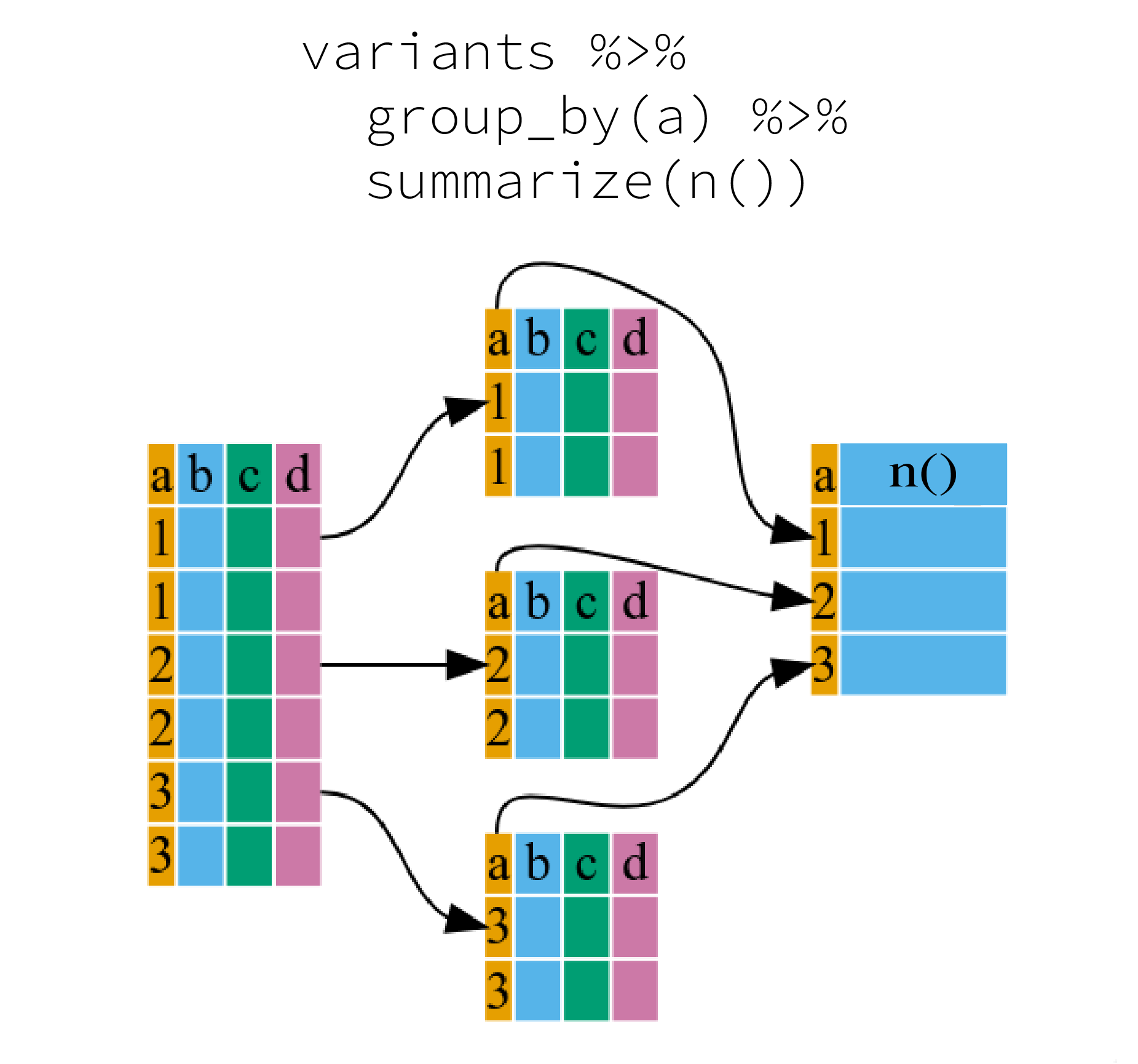
^[The figure was adapted from the Software Carpentry lesson, R for Reproducible Scientific Analysis]

Here the summary function used was n() to find the count for each group. Since this is a quite a common operation, there is a simpler method called tally():

variants %>%
  group_by(ALT) %>%
  tally()

# A tibble: 57 × 2
   ALT                                                          n
   <chr>                                                    <int>
A                                                          211
AC                                                           2
ACAGCCAGCCAGCCAGCCAGCCAGCCAGCCAGCCAG                         1
ACAGCCAGCCAGCCAGCCAGCCAGCCAGCCAGCCAGCCAGCCAGCCAGCCAGCCAG     1
ACCCCC                                                       2
ACCCCCCCC                                                    2
AGCGCGCGCG                                                   1
AGG                                                          1
AGGGGG                                                       2
AGGGGGG                                                      2
# … with 47 more rows

To show that there are many ways to achieve the same results, there is another way to approach this, which bypasses group_by() using the function count():

variants %>%
  count(ALT)

# A tibble: 57 × 2
   ALT                                                          n
   <chr>                                                    <int>
A                                                          211
AC                                                           2
ACAGCCAGCCAGCCAGCCAGCCAGCCAGCCAGCCAG                         1
ACAGCCAGCCAGCCAGCCAGCCAGCCAGCCAGCCAGCCAGCCAGCCAGCCAGCCAG     1
ACCCCC                                                       2
ACCCCCCCC                                                    2
AGCGCGCGCG                                                   1
AGG                                                          1
AGGGGG                                                       2
AGGGGGG                                                      2
# … with 47 more rows

Challenge

How many mutations are found in each sample?

Solution

variants %>%
  count(sample_id)

# A tibble: 3 × 2
  sample_id      n
  <chr>      <int>
1 SRR2584863    25
2 SRR2584866   766
3 SRR2589044    10

We can also apply many other functions to individual columns to get other summary statistics. For example,we can use built-in functions like mean(), median(), min(), and max(). These are called “built-in functions” because they come with R and don’t require that you install any additional packages. By default, all R functions operating on vectors that contains missing data will return NA. It’s a way to make sure that users know they have missing data, and make a conscious decision on how to deal with it. When dealing with simple statistics like the mean, the easiest way to ignore NA (the missing data) is to use na.rm = TRUE (rm stands for remove).

So to view the mean, median, maximum, and minimum filtered depth (DP) for each sample:

variants %>%
  group_by(sample_id) %>%
  summarize(
    mean_DP = mean(DP),
    median_DP = median(DP),
    min_DP = min(DP),
    max_DP = max(DP))

# A tibble: 3 × 5
  sample_id  mean_DP median_DP min_DP max_DP
  <chr>        <dbl>     <dbl>  <dbl>  <dbl>
1 SRR2584863    10.4      10        2     20
2 SRR2584866    10.6      10        2     79
3 SRR2589044     9.3       9.5      3     16

Reshaping data frames

It can sometimes be useful to transform the “long” tidy format, into the wide format. This transformation can be done with the pivot_wider() function provided by the tidyr package (also part of the tidyverse).

pivot_wider() takes a data frame as the first argument, and two arguments: the column name that will become the columns and the column name that will become the cells in the wide data.

variants_wide <- variants %>%
  group_by(sample_id, CHROM) %>%
  summarize(mean_DP = mean(DP)) %>%
  pivot_wider(names_from = sample_id, values_from = mean_DP)

`summarise()` has grouped output by 'sample_id'. You can override using the
`.groups` argument.

variants_wide

# A tibble: 1 × 4
  CHROM      SRR2584863 SRR2584866 SRR2589044
  <chr>           <dbl>      <dbl>      <dbl>
1 CP000819.1       10.4       10.6        9.3

The opposite operation of pivot_wider() is taken care by pivot_longer(). We specify the names of the new columns, and here add -CHROM as this column shouldn’t be affected by the reshaping:

variants_wide %>%
  pivot_longer(-CHROM, names_to = "sample_id", values_to = "mean_DP")

# A tibble: 3 × 3
  CHROM      sample_id  mean_DP
  <chr>      <chr>        <dbl>
1 CP000819.1 SRR2584863    10.4
2 CP000819.1 SRR2584866    10.6
3 CP000819.1 SRR2589044     9.3

Resources

Key Points

Use the dplyr package to manipulate data frames.

Use glimpse() to quickly look at your data frame.

Use select() to choose variables from a data frame.

Use filter() to choose data based on values.

Use mutate() to create new variables.

Use group_by() and summarize() to work with subsets of data.

previous episode

Intro to R and RStudio for Genomics

next episode

Data Wrangling and Analyses with Tidyverse

Overview

What is dplyr?

Taking a quick look at data frames

Selecting columns and filtering rows

Challenge

Solution

Challenge

Solution

Pipes

Exercise: Pipe and filter

Solution

Mutate

Exercise

Solution

group_by() and summarize() functions

Challenge

Solution

Reshaping data frames

Resources

Key Points

previous episode

next episode